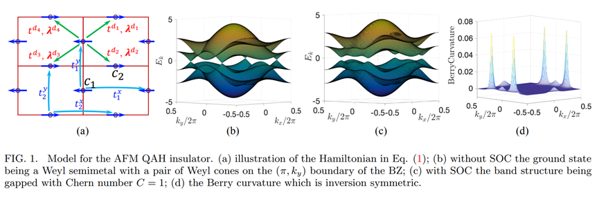
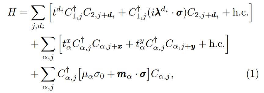
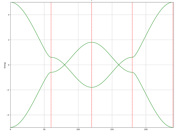
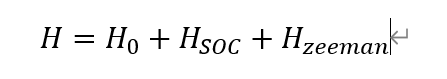
今天分享一篇arxiv上的文章:Guo P J, Liu Z X, Lu Z Y. Quantum anomalous Hall effect in antiferromagnetism[J]. arXiv preprint arXiv:2205.06702, 2022,揭示了反铁磁CrO中的量子反常霍尔效应,并给出了一个反铁磁的物理模型。我们来推导一下这个模型的结果。
from math import *
import math
import sys

from numpy import *

import matplotlib.pyplot as pl

# init K vector of random value

num = 2
knum = 241

lat_constant=1

Ham = [[0 for i in range(num)] for j in range(num)]

# print Ham
# exit()

mu = 0.6
t1=1
t2=0.6
t3=0.6


def H(kx, ky):
    # lattice
    Ham[0][0] = mu + t2*(exp(2*pi*complex(0,kx*lat_constant))+exp(2*pi*complex(0,-kx*lat_constant))) + t3*(exp(2*pi*complex(0,ky*lat_constant))+exp(2*pi*complex(0,-ky*lat_constant)))
    Ham[0][1] = t1*(exp(2*pi*complex(0,kx*0.5+ky*0.5)) + exp(2*pi*complex(0,kx*0.5-ky*0.5)) + exp(2*pi*complex(0,-kx*0.5+ky*0.5)) + exp(2*pi*complex(0,-kx*0.5-ky*0.5)))

    Ham[1][0] = Ham[0][1].conjugate()
    Ham[1][1] = -mu -t2*(exp(2*pi*complex(0,kx*lat_constant))+exp(2*pi*complex(0,-kx*lat_constant))) - t3*(exp(2*pi*complex(0,ky*lat_constant))+exp(2*pi*complex(0,-ky*lat_constant)))


    e, w = linalg.eig(Ham)
    e = [real(e[y]) for y in range(num)]
    e = sort(e)
    return e
    # for y in range(num):
    #     print real(e[y])
# H(0.01,0.03)
# exit()

ens = zeros((num, knum), dtype=float64)
a1 = open("kpoints", 'r+')      #Using Fractional coordinates
for m in range(knum):
    Kq = a1.readline().strip().split()
    kx,ky=[float(Kq[n]) for n in range(2)]
    e=H(kx,ky)
    for y in range(num):
      ens[y, m] = real(e[y])
print(ens)


pl.figure(figsize=(16.0, 12.4))
pl.subplots_adjust(wspace=0.35)
pl.ylim(-5,5)
pl.xlim(0, knum)
pl.grid(True)

# print(nOrbits)
for i in range(num):
    # print i
    # pl.plot(ens[i], 'go', ms=5, mew=1)
    pl.plot(ens[i], 'g-', ms=5, mew=1)
    # pl.plot(evals[i], 'ro', ms=5, mew=1)
pl.title(r'$\Gamma$')

pl.ylabel("Energy")
vline_indx = [60,120,180,240]
pl.vlines(vline_indx, -100, 100, colors='r', linestyles='dashed', label='垂直线')

pl.show()

print('Done.\n')
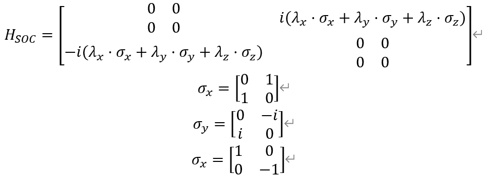
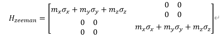
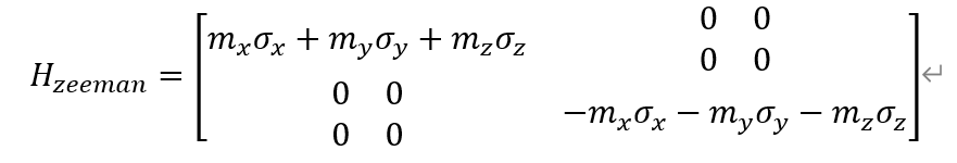
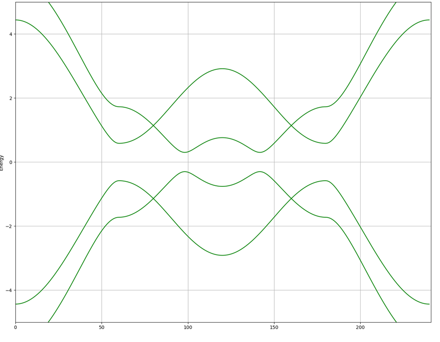
考虑SOC及赛曼场的作用,
from math import *
import math
import sys
from numpy import *
import matplotlib.pyplot as pl
from mpl_toolkits.mplot3d import Axes3D
# init K vector of random value
num = 4
knum = 241
lat_constant=1
Ham = [[0 for i in range(num)] for j in range(num)]
# print Ham
# exit()
mu = 0.6
t1=1
t2=0.6
t3=0.6
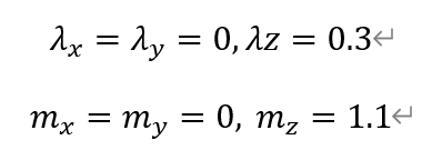
lam=0.3
mz=1.1
def H(kx, ky):
# lattice
Ham[0][0] = mu + t2*(exp(2*pi*complex(0,kx*lat_constant))+exp(2*pi*complex(0,-kx*lat_constant))) + t3*(exp(2*pi*complex(0,ky*lat_constant))+exp(2*pi*complex(0,-ky*lat_constant))) +mz
Ham[1][1] = mu + t2*(exp(2*pi*complex(0,kx*lat_constant))+exp(2*pi*complex(0,-kx*lat_constant))) + t3*(exp(2*pi*complex(0,ky*lat_constant))+exp(2*pi*complex(0,-ky*lat_constant))) -mz
Ham[0][1]=0
Ham[1][0]=0
Ham[0][2] = t1*(exp(2*pi*complex(0,kx*0.5+ky*0.5)) + exp(2*pi*complex(0,kx*0.5-ky*0.5)) + exp(2*pi*complex(0,-kx*0.5+ky*0.5)) + exp(2*pi*complex(0,-kx*0.5-ky*0.5))) + complex(0,lam)
Ham[1][3] = t1*(exp(2*pi*complex(0,kx*0.5+ky*0.5)) + exp(2*pi*complex(0,kx*0.5-ky*0.5)) + exp(2*pi*complex(0,-kx*0.5+ky*0.5)) + exp(2*pi*complex(0,-kx*0.5-ky*0.5))) - complex(0,lam)
Ham[0][3] = 0
Ham[1][2] = 0
Ham[2][0] = Ham[0][2].conjugate()
Ham[2][1] = 0
Ham[3][0] = 0
Ham[3][1] = Ham[1][3].conjugate()
Ham[2][2] = -mu -t2*(exp(2*pi*complex(0,kx*lat_constant))+exp(2*pi*complex(0,-kx*lat_constant))) - t3*(exp(2*pi*complex(0,ky*lat_constant))+exp(2*pi*complex(0,-ky*lat_constant))) -mz
Ham[3][3] = -mu -t2*(exp(2*pi*complex(0,kx*lat_constant))+exp(2*pi*complex(0,-kx*lat_constant))) - t3*(exp(2*pi*complex(0,ky*lat_constant))+exp(2*pi*complex(0,-ky*lat_constant))) +mz
Ham[2][3] = 0
Ham[3][2] = 0
e, w = linalg.eig(Ham)
e = [real(e[y]) for y in range(num)]
e = sort(e)
return e
# for y in range(num):
# print real(e[y])
# H(0.01,0.03)
# exit()
ens = zeros((num, knum), dtype=float64)
a1 = open("kpoints", 'r+') #Using Fractional coordinates
for m in range(knum):
Kq = a1.readline().strip().split()
kx,ky=[float(Kq[n]) for n in range(2)]
e=H(kx,ky)
for y in range(num):
ens[y, m] = real(e[y])
print(ens)
pl.figure(figsize=(16.0, 12.4))
pl.subplots_adjust(wspace=0.35)
pl.ylim(-5,5)
pl.xlim(0, knum)
pl.grid(True)
# print(nOrbits)
for i in range(num):
# print i
# pl.plot(ens[i], 'go', ms=5, mew=1)
pl.plot(ens[i], 'g-', ms=5, mew=1)
# pl.plot(evals[i], 'ro', ms=5, mew=1)
pl.title(r'$\Gamma$')
pl.ylabel("Energy")
# pl.show()
# print('Done.\n')
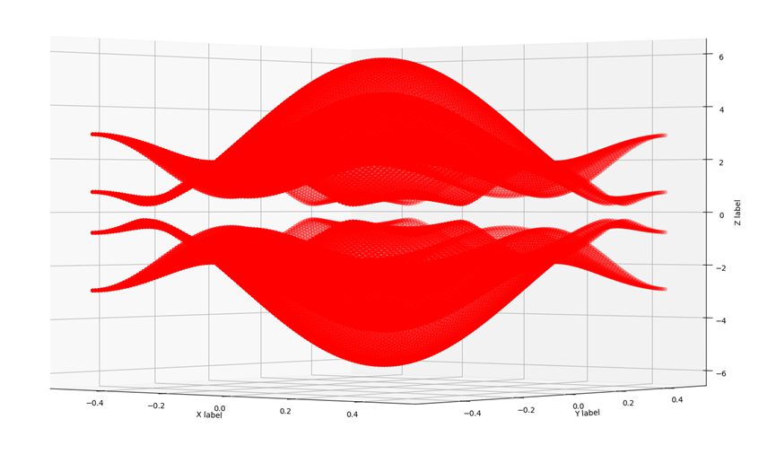
fig = pl.figure() # 创建一个画布figure,然后在这个画布上加各种元素。
ax = Axes3D(fig) # 将画布作用于 Axes3D 对象上。
a=arange(-0.5,0.5,0.01)
x=zeros((1, 100),dtype=float64)
y=zeros((1, 100),dtype=float64)
z0=zeros((1,100),dtype=float64)
z1=zeros((1,100),dtype=float64)
z2=zeros((1,100),dtype=float64)
z3=zeros((1,100),dtype=float64)
for i in range(len(a)):
kx=a[i]
x[0,]=kx
for j in range(len(a)):
ky=a[j]
y[0,j]=ky
e=H(kx,ky)
z0[0, j] = real(e[0])
z1[0, j] = real(e[1])
z2[0, j] = real(e[2])
z3[0, j] = real(e[3])
ax.scatter(x,y,z0,c='r') # 画出(xs1,ys1,zs1)的散点图。
ax.scatter(x,y,z1,c='r') # 画出(xs1,ys1,zs1)的散点图。
ax.scatter(x,y,z2,c='r') # 画出(xs1,ys1,zs1)的散点图。
ax.scatter(x,y,z3,c='r') # 画出(xs1,ys1,zs1)的散点图。
ax.set_xlabel('X label') # 画出坐标轴
ax.set_ylabel('Y label')
ax.set_zlabel('Z label')
pl.show()


No Comments
Leave a comment Cancel